Friday 12 December 2014

the first BKO claim:

And now, what I have been building to, the first big claim for the BKO scheme:
"all finite relatively static knowledge can be represented in the BKO scheme"

If I was a real computer scientist or mathematician I would prove that claim. But I'm a long way from that, so the best I can offer is, "it seems to be the case with the examples I have tried so far". Yeah, vastly unsatisfying compared to a real proof.

And a couple of notes:
1) BKO is what I call an "active representation". Once in this format a lot of things are relatively easy. eg, working with the IMDB data was pretty much trivial.
2) One of the driving forces behind BKO is to try and collapse all knowledge into one general/unified representation (OP KET => SUPERPOSITION). The benefit being that if you develop machinery for one branch of knowledge it often extends easily to other branches.
3) The next driving force is efficiency of the notation. So while my results are possible to reproduce using other methods, BKO notation is more efficient. One benefit of the correct notation is if you make a hard thing easier, you in turn make a harder thing possible. eg, in physics there are notational short-cuts all over the place for just this reason.
4) Another selling point for the BKO notation is how closely English maps to it.

How about a summary of some examples that show how clean and powerful the notation is:
Learning plurals:
plural |word: *> #=> merge-labels(|_self> + |s>)
plural |word: foot> => |word: feet>
plural |word: mouse> => |word: mice>
plural |word: radius> => |word: radii>
plural |word: tooth> => |word: teeth>
plural |word: person> => |word: people> 
Some general rules that apply to all people:
siblings |person: *> #=> brothers |_self> + sisters |_self>
children |person: *> #=> sons |_self> + daughters |_self>
parents |person: *> #=> mother |_self> + father |_self>
uncles |person: *> #=> brothers parents |_self>
aunts |person: *> #=> sisters parents |_self>
aunts-and-uncles |person: *> #=> siblings parents |_self>
cousins |person: *> #=> children siblings parents |_self>
grand-fathers |person: *> #=> father parents |_self>
grand-mothers |person: *> #=> mother parents |_self>
grand-parents |person: *> #=> parents parents |_self>
grand-children |person: *> #=> children children |_self>
great-grand-parents |person: *> #=> parents parents parents |_self>
great-grand-children |person: *> #=> children children children |_self>
immediate-family |person: *> #=> siblings |_self> + parents |_self> + children |_self>
friends-and-family |person: *> #=> friends |_self> + family |_self>
Asking about Fred:
"Who are Fred's friends?"
friends |Fred>

"What age are Fred's friends?"
age friends |Fred>

"How many friends does Fred have?"
how-many friends |Fred>

"Do you know the age of Fred's friends?"
do-you-know age friends |Fred>

"Who are Fred's friends of friends?"
friends friends |Fred>

"What age are Fred's friends of friends?"
age friends friends |Fred>

"How many friends of friends does Fred have?"
how-many friends friends |Fred>
... and so on. 
Some movie trivia:
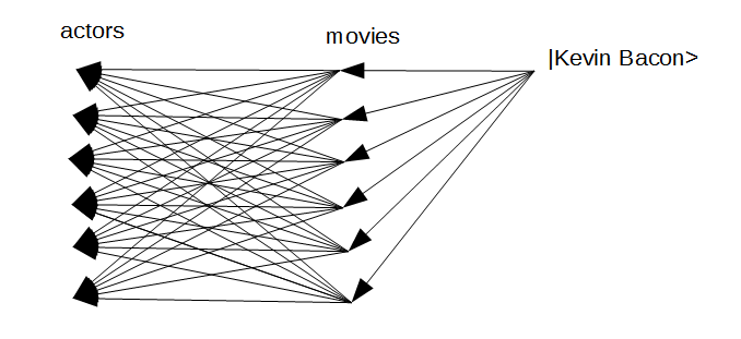
"What movies do Matt Damon and Morgan Freeman have in common?"
common[movies] (|actor: Matt Damon> + |actor: Morgan (I) Freeman>)
movie: Invictus (2009)
movie: The People Speak (2009)
movie: Magnificent Desolation: Walking on the Moon 3D (2005)

"What actors do "Ocean's Twelve" and "Ocean's Thirteen" have in common?"
common[actors] (|movie: Ocean's Twelve (2004)> + |movie: Ocean's Thirteen (2007)> )
actor: Don Cheadle
actor: Casey Affleck
actor: Elliott Gould
actor: Bernie Mac
actor: Matt Damon
actor: Brad Pitt
actor: Eddie Izzard
actor: Eddie Jemison
actor: George Clooney
actor: Scott Caan
actor: Jerry (I) Weintraub
actor: Scott L. Schwartz
actor: Carl Reiner
actor: Shaobo Qin
actor: Andy (I) Garcia
actor: Vincent Cassel
Kevin Bacon numbers:
kevin-bacon-0 |result> => |actor: Kevin (I) Bacon> 
kevin-bacon-1 |result> => actors movies |actor: Kevin (I) Bacon>
kevin-bacon-2 |result> => [actors movies]^2 |actor: Kevin (I) Bacon>
kevin-bacon-3 |result> => [actors movies]^3 |actor: Kevin (I) Bacon>
kevin-bacon-4 |result> => [actors movies]^4 |actor: Kevin (I) Bacon>
Working with a grid:
sa: load 45-by-45-grid.sw
sa: near |grid: *> #=> |_self> + N|_self> + NE|_self> + E|_self> + SE|_self> + S|_self> + SW|_self> + W|_self> + NW|_self>
sa: building |grid: 4 40> => |building: cafe>
sa: create inverse
sa: current |location> => inverse-building |building: cafe>

-- now ask what is your current location?
sa: current |location>
|grid: 4 40>

-- what is near your current location?
sa: near current |location>
|grid: 4 40> + |grid: 3 40> + |grid: 3 41> + |grid: 4 41> + |grid: 5 41> + |grid: 5 40> + |grid: 5 39> + |grid: 4 39> + |grid: 3 39>

-- what is 3 steps NW of your current location?
sa: NW^3 current |location>
|grid: 1 37>

-- what is near 3 steps NW of your current location?
-- NB: since we are at the edge of a finite universe grid, there are less neighbours than in other examples of near.
-- this BTW, makes use of |> as the identity element for superpositions
sa: near NW^3 current |location>
|grid: 1 37> + |grid: 1 38> + |grid: 2 38> + |grid: 2 37> + |grid: 2 36> + |grid: 1 36>

-- what is 7 steps S of your current location?
sa: S^7 current |location>
|grid: 11 40>

-- what is near 7 steps S of your current location?
sa: near S^7 current |location>
|grid: 11 40> + |grid: 10 40> + |grid: 10 41> + |grid: 11 41> + |grid: 12 41> + |grid: 12 40> + |grid: 12 39> + |grid: 11 39> + |grid: 10 39>
Working with ages:
age-1 |age: *> #=> arithmetic(|_self>,|->,|age: 1>)
age+1 |age: *> #=> arithmetic(|_self>,|+>,|age: 1>)
almost |age: *> #=> age-1 |_self>
roughly |age: *> #=> 0.5 age-1 |_self> + |_self> + 0.5 age+1 |_self>

-- almost 19:
sa: almost |age: 19>
|age: 18>

-- roughly 27:
sa: roughly |age: 27>
0.500|age: 26> + |age: 27> + 0.500|age: 28>
Learning indirectly:
-- set our "you" variable:
sa: |you> => |Sam>
-- learn your age:
sa: age "" |you> => |age: 23>

-- ask Sam's age:
sa: age |Sam>
|age: 23>

-- greet you:
sa: random-greet "" |you>
|Good morning Sam.>
And that pretty much concludes phase 1 of my write-up. Heaps more to come!

Update: here is a fun example of the right notation making things easier.
Consider algebra, but using Roman not Arabic numerals:
27x^3 + 78y + 14
vs:
XXVII * x^3 + LXXVIII * y + XIV
or alternatively consider trying to read a large matrix with values written in Roman numerals. Ouch!

Update: we can do all the above examples using just these key pieces:
OP KET => SUPERPOSITION
label descent, eg: |word: *>, |person: *>, |grid: *>, |age: *>
stored rules, ie: #=>
merge-labels()
|_self>
common[OP] (|x> + |y>)
load file.sw
create inverse
|> as the identity element for superpositions
arithmetic()
learning indirectly, eg: age "" |you> => |age: 27>
pick-elt (inside random-greet)

Thursday 11 December 2014

the maths rules for the BKO scheme

Here are the maths rules behind BKO:
1) <x||y> == 0 if x != y.  
2) <x||y> == 1 if x == y.
3) <!x||y> == 1 if x != y. (NB: the ! acts as a not. cf, the -v switch for grep) 
4) <!x||y> == 0 if x == y.
5) <x: *||y: z> == 0 if x != y.
6) <x: *||y: z> == 1 if x == y, for any z. 
7) applying bra's is linear. <x|(|a> + |b> + |c>) == <x||a> + <x||b> + <x||c>
8) if a coeff is not given, then it is 1. eg, <x| == <x|1 and 1|x> == |x>
9) bra's and ket's commute with the coefficients. eg, <x|7 == 7 <x| and 13|x> == |x>13  
10) in contrast to QM, in BKO operators are right associative only.
<a|(op|b>) is valid and is identical to <a|op|b>
(<a|op)|b> is invalid, and undefined.
11) again, in contrast to QM, <a|op|b> != <b|op|a>^* (a consequence of (10) really)
12) applying projections is linear. |x><x|(|a> + |b> + |c>) == |x><x||a> + |x><x||b> + |x><x||c>
13) kets in superpositions commute. |a> + |b> == |b> + |a>
14) kets in sequences do not commute. |a> . |b> != |b> . |a>
Though maybe in the sequence version of simm, this would be useful:
|a> . |b> = c |b> . c |a>, where usually c is < 1. (yeah, it "bugs out" if you swap it back again, but in practice should be fine)
another example: 
  |c> . |a> . |b> = c |a> . c |c> . |b>
                  = c |a> . c |b> . c^2 |c>
15) operators (in general) do not commute. <b|op2 op1|a> != <b|op1 op2|a>
16) if a coeff in a superposition is zero, we can drop it from the superposition without changing the meaning of that superposition. 
17) we can arbitrarily add kets to a superposition if they have coeff zero without changing the meaning of that superposition.
18) |> is the identity element for superpositions. sp + |> == |> + sp == sp.
19) the + sign in superpositions is literal. ie, kets add.
|a> + |a> + |a> = 3|a>
|a> + |b> + |c> + 6|b> = |a> + 7|b> + |c>
20) <x|op-sequence|y> is always a scalar/float
21) |x><x|op-sequence|y> is always a ket or a superposition

some bigger sw examples

Now we have most of the basics out of the way, we can look at some bigger examples.
So here are several public databases that I have mapped to sw format:

GeoNames
"The GeoNames geographical database covers all countries and contains over eight million placenames that are available for download free of charge."
http://www.geonames.org/
And my rough version of the Australian data here (yeah, I want to redo at some stage):
geonames-au-id-version.sw (50 MB,  7 op types and 871,186 learn rules)
improved sw versions:
improved-geonames-au.sw (109 MB, 11 op types and 1,544,996 learn rules)
improved-geonames-cities-1000.sw (94 MB, 11 op types and 1,375,844 learn rules)
improved-geonames-cities-15000.sw (17 MB, 11 op types and 236,184 learn rules)
improved-geonames-de.sw (99 MB, 11 op types and 1,454,997 learn rules)
improved-geonames-fr.sw (83 MB, 11 op types and 1,203,510 learn rules)
improved-geonames-gb.sw (31 MB, 11 op types and 441,431 learn rules)
improved-geonames-us.sw (1.3 GB, 11 op types and 18,950,003 learn rules)

Moby Thesaurus
"Moby Thesaurus is the largest and most comprehensive thesaurus data source in English available for commercial use. This second edition has been thoroughly revised adding more than 5,000 root words (to total more than 30,000) with an additional million synonyms and related terms (to total more than 2.5 million synonyms and related terms)."
http://icon.shef.ac.uk/Moby/mthes.html
Again, my rough version here:
moby-thesaurus.sw (32 MB, 1 op type and 30,244 learn rules)
improved sw version:
improved-moby-thesaurus.sw (50 MB, 1 op type and 30,260 learn rules)

Moby Part-of-Speech
"This second edition is a particularly thorough revision of the original Moby Part-of-Speech. Beyond the fifteen thousand new entries, many thousand more entries have been scrutinized for correctness and modernity. This is unquestionably the largest P-O-S list in the world."
http://icon.shef.ac.uk/Moby/mpos.html
The sw version:
part-of-speech.sw (16 MB, 1 op type and 233,090 learn rules)

Frequently Occurring Surnames from Census 1990
http://www.census.gov/topics/population/genealogy/data/1990_census/1990_census_namefiles.html#
The sw version:
names.sw (1.7 MB,  1 op type and 4 learn rules)

IMDB database:
ftp://ftp.fu-berlin.de/pub/misc/movies/database/
The sw version:
improved-imdb.sw (588 MB, 2 op types and 2,591,132 learn rules)
imdb-ratings.sw (1.6 MB, 4 op types and 21,820 learn rules)
improved-imdb-year.sw (470 MB, 4 op types and 3,146,301 learn rules)

A year's worth of historical share data (I forget the source!)
shares.sw (17 MB, 5 op types and 2,622 learn rules)

And I guess that is about it. The only note I want to make is that in each of these examples I had to write a custom script to parse! Once in sw format, parsing is trivial and identical in each case. Yeah, I'm trying to push my sw notation! I certainly think it is superior to XML.

Update: in a future phase of the project I would like to extend this, and map even more data sets to sw format.

Update: I now have a script to produce the stats summary of sw files.

finding common movies and actors

We can have a lot of fun with the imdb data. This time, given two actors, find which movies they shared. Alternatively, given two movies, find the common actors.

Let's jump right into the python:
#!/usr/bin/env python3

import sys

if len(sys.argv) < 3:
  print("\nUsage:")
  print("  ./find_common.py actor1 actor2")
  print("  ./find_common.py movie1 movie2\n")
  sys.exit(0)

one = sys.argv[1]
two = sys.argv[2]

def file_recall(filename,op,label):
  pattern = op + " |" + label + "> => "
  n = len(pattern)
  with open(filename,'r') as f:
    for line in f:
      if line.startswith(pattern):
        line = line[n:]
        return line[1:-1].split("> + |")
  return []

def display(line):
#  return ", ".join(line)
  return "\n".join(line)

def intersection(a,b):
  return list(set(a) & set(b))

imdb_sw = "sw-examples/improved-imdb.sw"    # our imdb data

def print_common_movies(sw_file,one,two):
  actor1 = "actor: " + one
  actor2 = "actor: " + two
  movies1 = file_recall(sw_file,"movies",actor1)
  movies2 = file_recall(sw_file,"movies",actor2)

# check if we have info on them:
  if len(movies1) == 0 or len(movies2) == 0:
    return

  common_movies = intersection(movies1,movies2)

  print()
  print("common movies for:")
  print(one)
  print(two)
  print("number of common movies:",len(common_movies))
  print("common movies:")
  print(display(common_movies))
  print()

def print_common_actors(sw_file,one,two):
  movie1 = "movie: " + one
  movie2 = "movie: " + two
  actors1 = file_recall(sw_file,"actors",movie1)
  actors2 = file_recall(sw_file,"actors",movie2)

# check if we have info on them:
  if len(actors1) == 0 or len(actors2) == 0:
    return

  common_actors = intersection(actors1,actors2)

  print()
  print("common actors for:")
  print(one)
  print(two)
  print("number of common actors:",len(common_actors))
  print("common actors:")
  print(display(common_actors))
  print()


print_common_actors(imdb_sw,one,two)
print_common_movies(imdb_sw,one,two)
Now some examples:
$ ./find_common.py "Tom Cruise" "Nicole Kidman"

common movies for:
Tom Cruise
Nicole Kidman
number of common movies: 8
common movies:
movie: Eyes Wide Shut (1999)
movie: Days of Thunder (1990)
movie: Der Geist des Geldes (2007)
movie: August (2008)
movie: Boffo! Tinseltown's Bombs and Blockbusters (2006)
movie: Stanley Kubrick: A Life in Pictures (2001)
movie: Far and Away (1992)
movie: The Queen (2006)


$ ./find_common.py "Matt Damon" "Morgan (I) Freeman"

common movies for:
Matt Damon
Morgan (I) Freeman
number of common movies: 3
common movies:
movie: Invictus (2009)
movie: The People Speak (2009)
movie: Magnificent Desolation: Walking on the Moon 3D (2005)

$ ./find_common.py "Bruce Willis" "Tom Cruise"

common movies for:
Bruce Willis
Tom Cruise
number of common movies: 1
common movies:
movie: Boffo! Tinseltown's Bombs and Blockbusters (2006)

$ ./find_common.py "Bruce Willis" "Matt Damon"

common movies for:
Bruce Willis
Matt Damon
number of common movies: 1
common movies:
movie: Ocean's Twelve (2004)

$ ./find_common.py "Brad Pitt" "George Clooney"

common movies for:
Brad Pitt
George Clooney
number of common movies: 7
common movies:
movie: Burn After Reading (2008)
movie: Ocean's Twelve (2004)
movie: Boffo! Tinseltown's Bombs and Blockbusters (2006)
movie: Ocean's Eleven (2001)
movie: Touch of Evil (2011)
movie: Ocean's Thirteen (2007)
movie: Confessions of a Dangerous Mind (2002)

$ ./find_common.py "Matt Damon" "Ben Affleck"

common movies for:
Matt Damon
Ben Affleck
number of common movies: 10
common movies:
movie: Chasing Amy (1997)
movie: Jersey Girl (2004)
movie: Jay and Silent Bob Strike Back (2001)
movie: School Ties (1992)
movie: Glory Daze (1995)
movie: Dogma (1999)
movie: The Third Wheel (2002)
movie: Good Will Hunting (1997)
movie: Unite for Japan (2011)
movie: Field of Dreams (1989)

-- now find the common actors for the Ocean's series of movies:
$ ./find_common.py "Ocean's Eleven (2001)" "Ocean's Twelve (2004)"

common actors for:
Ocean's Eleven (2001)
Ocean's Twelve (2004)
number of common actors: 18
common actors:
actor: David (II) Sontag
actor: Casey Affleck
actor: Julia (I) Roberts
actor: Andy (I) Garcia
actor: George Clooney
actor: Eddie Jemison
actor: Elliott Gould
actor: Larry Sontag
actor: Matt Damon
actor: Carl Reiner
actor: Topher Grace
actor: Brad Pitt
actor: Scott L. Schwartz
actor: Scott Caan
actor: Bernie Mac
actor: Jerry (I) Weintraub
actor: Shaobo Qin
actor: Don Cheadle

$ ./find_common.py "Ocean's Twelve (2004)" "Ocean's Thirteen (2007)"

common actors for:
Ocean's Twelve (2004)
Ocean's Thirteen (2007)
number of common actors: 16
common actors:
actor: Don Cheadle
actor: Casey Affleck
actor: Elliott Gould
actor: Bernie Mac
actor: Matt Damon
actor: Brad Pitt
actor: Eddie Izzard
actor: Eddie Jemison
actor: George Clooney
actor: Scott Caan
actor: Jerry (I) Weintraub
actor: Scott L. Schwartz
actor: Carl Reiner
actor: Shaobo Qin
actor: Andy (I) Garcia
actor: Vincent Cassel
So that was all kinda fun! I guess the only note is I was thinking of implementing a google like "did you mean", because currently if you don't get the actor or movie name exactly right, you don't get any results. Shouldn't be too hard to implement something like that.

Update: IMDB does something similar too, which isn't really surprising.

Update: Here are a bunch of other results using the IMDB data:
all-actors-average.txt
all-actors-weighted-average.txt
movie-only-votes-ratings-title.txt
sorted-all-actors-average.txt
sorted-all-actors-weighted-average.txt
sorted-top-1000-actors-average.txt
sorted-top-1000-actors-weighted-average.txt
star-studded-movies.txt
top-1000-actors-average.txt
top-1000-actors-weighted-average.txt
top-1000-actors.txt
top-2500-well-known-actors.txt
votes-ratings-title.txt
well-known-actors.txt
kevin-bacon-numbers.sw

Kevin Bacon game/numbers

Now we have a copy of IMDB movie and actor data in sw format (which BTW, we created using data from here) we can use that for the Kevin Bacon game and Kevin Bacon numbers. See WP for their definition.

In our notation, we can find actors Kevin Bacon numbers using something like:
kevin-bacon-0 |result> => |actor: Kevin (I) Bacon> 
kevin-bacon-1 |result> => actors movies |actor: Kevin (I) Bacon>
kevin-bacon-2 |result> => [actors movies]^2 |actor: Kevin (I) Bacon>
kevin-bacon-3 |result> => [actors movies]^3 |actor: Kevin (I) Bacon>
kevin-bacon-4 |result> => [actors movies]^4 |actor: Kevin (I) Bacon>
... and so on.
And visually looks something like this:

So, easy enough in theory but too slow to do that directly, so we drop back to using file_recall().
The python is not too hard:
# a single layer of the Kevin Bacon game.
# one is a superposition (though should handle kets too)
# returns a superposition.
#
# the code does: 
#   actors movies SUPERPOSITION
# eg: 
#   actors movies |actor: Kevin (I) Bacon>
#
def Kevin_Bacon_game(bacon_file,one):
  if type(one) == str:                   # make sure we have a superposition,
    one = superposition() + ket(one)     # even if fed a string or a ket
  elif type(one) == ket:                 # Hrmm... there has to be a neater way to write this mess!
    one = superposition() + one

#  one = one.apply_sigmoid(clean)         # optional to clean coeffs from our incoming sp

  sp1 = superposition()
  for x in one.data:
    sp1 += file_recall(bacon_file,"movies",x)

  sp2 = superposition()
  for x in sp1.data:
    sp2 += file_recall(bacon_file,"actors",x)

  print("len:",len(sp2))
  return sp2.coeff_sort()


sw_bacon_file = "sw-examples/improved-imdb.sw"    # our imdb data
r = ket("actor: Kevin (I) Bacon")                 # NB: we can choose any actor we like! We have the whole imdb to choose from!
N = 2                                             # How deep we want to go. For now 2, but maybe 4 or bigger later!
for k in range(N):
  r = Kevin_Bacon_game(sw_bacon_file,r)
  C.learn("kevin-bacon-" + str(k + 1),"result",r)

name = "sw-examples/kevin-bacon.sw"               # save the results.
save_sw(C,name)
Indeed, even that might be too slow. So another optimization, we write to disk as we go:
# let's write a version that writes to disk as it goes.
sw_bacon_file = "sw-examples/improved-imdb.sw"    # our imdb data
sw_dest_file = "sw-examples/fast-write--kevin-bacon.sw" # where we are going to save the results
dest = open(sw_dest_file,'w')

# write the context header:
dest.write("|context> => |context: Kevin Bacon game>\n\n")

r = ket("actor: Kevin (I) Bacon")                    # NB: we can choose any actor we like! We have the whole imdb to choose from!
N = 2                                                # How deep we want to go. For now 2, but maybe 4 or bigger later.
for k in range(N):
  r = Kevin_Bacon_game(sw_bacon_file,r)
  dest.write("kevin-bacon-" + str(k+1) + " |result> => " + r.display(True) + "\n")  # r.display(True) for exact dump, not str(sp) version.
dest.close()
And here is the resulting kevin-bacon.sw file.

Now, a couple of notes:
1) superposition += is O(n^2) or something! This is because superpositions are (currently) lists, and when you add a superposition to a superposition you have to walk the entire list checking if those kets are already in the list. Anyway, that is why I'm thinking of swapping superpositions to ordered dictionaries (note we can't use standard dictionaries because we do want to keep some sense of order even if technically kets in superpositions commute). Anyway, this is a big problem all over the place, and I've been writing hacks (eg, one of those hacks is working with dictionaries, and then when finished map that to a superposition, this drops it back to O(n) and makes a massive speed difference) to step around it for ages now. So how big of a problem is it? Well, in the current case N = 1 took 1 minute, N = 2 took 12 days! So we haven't even tried for bigger N.
2) Turns out that the number of pathways between Kevin Bacon via [actors movies] to an actor, somehow selects out well known actors. Not sure if that is because I used an older imdb data set that didn't fully filter out TV shows, and in particular award shows (that over represent well known actors), or if it is a more general thing. Anyway, this should show what I mean:
$ grep "^kevin-bacon-1 " ec2-fast-write--kevin-bacon.sw | sed 's/=> /\n/g' | sed 's/ + /\n/g' | head -30
kevin-bacon-1 |result>
182.0|actor: Kevin (I) Bacon>
30.0|actor: Kyra Sedgwick>
22.0|actor: Tom Hanks>
15.0|actor: Meryl Streep>
15.0|actor: Tina Fey>
14.0|actor: George Clooney>
14.0|actor: Drew (I) Barrymore>
13.0|actor: Clint Eastwood>
12.0|actor: Sandra Bullock>
12.0|actor: Alec Baldwin>
12.0|actor: Steve Carell>
12.0|actor: Laurence Fishburne>
12.0|actor: Brad Pitt>
12.0|actor: Kevin Spacey>
11.0|actor: Leonardo DiCaprio>
11.0|actor: Kiefer Sutherland>
11.0|actor: Amy Poehler>
11.0|actor: Tom Cruise>
11.0|actor: Michael (I) Douglas>
11.0|actor: Tim (I) Robbins>
10.0|actor: Morgan (I) Freeman>
10.0|actor: Candice Bergen>
10.0|actor: Eva Longoria>
10.0|actor: Matt Damon>
10.0|actor: Susan Sarandon>
10.0|actor: Hugh Laurie>
10.0|actor: Mark (I) Wahlberg>
10.0|actor: Glenn Close>
10.0|actor: Jennifer Love Hewitt>

$ grep "^kevin-bacon-2 " ec2-fast-write--kevin-bacon.sw | sed 's/=> /\n/g' | sed 's/ + /\n/g' | head -30
kevin-bacon-2 |result>
58714.0|actor: Kevin (I) Bacon>
41662.0|actor: Tom Hanks>
29505.0|actor: Meryl Streep>
28364.0|actor: Steven Spielberg>
27638.0|actor: George Clooney>
27622.0|actor: Nicole Kidman>
25941.0|actor: Michael (I) Douglas>
25214.0|actor: Alec Baldwin>
24562.0|actor: Tina Fey>
24535.0|actor: Samuel L. Jackson>
23908.0|actor: Clint Eastwood>
23795.0|actor: Dustin Hoffman>
23746.0|actor: Halle Berry>
23337.0|actor: Glenn Close>
23018.0|actor: Morgan (I) Freeman>
22977.0|actor: Brad Pitt>
22892.0|actor: Susan Sarandon>
22818.0|actor: Drew (I) Barrymore>
22574.0|actor: Kevin Spacey>
22469.0|actor: Helen Mirren>
22394.0|actor: Kyra Sedgwick>
22290.0|actor: Tom Cruise>
22033.0|actor: John Travolta>
21936.0|actor: Leonardo DiCaprio>
21578.0|actor: Sandra Bullock>
20835.0|actor: Whoopi Goldberg>
20533.0|actor: Will (I) Smith>
20262.0|actor: Jennifer (I) Lopez>
20199.0|actor: Robin (I) Williams>
Again, neat! Notice how they are all well known actors. Interesting that this just fell out.

3) Quick look at how many actors are in Kevin-Bacon-k:
-- how many movies in the full imdb.sw file:
$ grep -c "^actors |movie: " imdb.sw
770170

-- how many actors in the full imdb.sw file:
$ grep -c "^movies |actor: " imdb.sw
2436366

-- how many actors in kevin-bacon-1:
$ grep "^kevin-bacon-1 " ec2-fast-write--kevin-bacon.sw | sed 's/=> /\n/g' | sed 's/ + /\n/g' | wc -l
6244

-- how many actors in kevin-bacon-2:
$ grep "^kevin-bacon-2 " ec2-fast-write--kevin-bacon.sw | sed 's/=> /\n/g' | sed 's/ + /\n/g' | wc -l
655902
4) Now a comment on sw format vs a matrix representation of the same.
Consider:
kevin-bacon-1 |result> => actors movies |actor: Kevin (I) Bacon>
Well, if we did the same thing using matrices, and yeah, this maps trivially to a matrix representation, it would be expensive. The input vector would be 2,436,366 long, and the [actors movies] matrix would be 2,436,366 * 2,436,366. ie, 5,935,879,285,956 elements. Ouch!

That's it for now. More imdb related in the next post!

Update: this is related: The Oracle of Bacon

Wednesday 10 December 2014

introducing file_recall()

So, with small files it is fine to use the standard:
context.recall(op,label)
but once you start working with large sw files, it is prohibitively slow to load the entire sw file into memory, then work on it, then spit out your result. I'm talking days here for the improved-imdb.sw file.
The fix is this function:
# filename is sw data/source file
# op is the operator label, a string
# label is the ket label, a string or a ket
#
# returns a superposition
def file_recall(filename,op,label):
  if type(label) == ket:
    coeff = label.value
    ket_label = label.label
  else:
    coeff = 1
    ket_label = label

  pattern = op + " |" + ket_label + "> => "
  n = len(pattern)
#  print("pattern:",pattern)
#  print("n:      ",n)

  with open(filename,'r') as f:
    for line in f:
      if line.startswith(pattern):
        return extract_literal_superposition(line[n:])[0].multiply(coeff)
  return ket("",0)

And we can tweak this. If all superpositions in your sw file are "clean superpositions". Yeah, a term I just made up. But what I mean is:
if all coeffs in our superposition are 1, and implicit, we can call it a "clean superposition"
So: |a> + |b> + |c> is a clean superposition, and 3|a> + |b> + 21|d> is not.

And if we also have op and label are always strings, then we can simplify the file_recall() code down to this (which BTW returns a list and not a superposition):
def file_recall(filename,op,label):
  pattern = op + " |" + label + "> => "
  n = len(pattern)
  with open(filename,'r') as f:
    for line in f:
      if line.startswith(pattern):
        line = line[n:]
        return line[1:-1].split("> + |")
  return []

Anyway, we make use of file_recall() in the next couple of posts.
And a couple of notes:
1) often you can drastically speed up processing of large sw files by grepping down to the rule-types of interest. eg:
grep "^op " example-file.sw
2) maybe one day make the in-memory/in-file distinction transparent to the working code? I don't yet know if that is a good idea or not.
3) note how simple the second file_recall() code is! This is another win from our simple sw notation:
OP KET => SUPERPOSITION

context.recall() vs x.apply_op()

Now, here is a key part of the project that I haven't mentioned yet (though there are plenty of others!). We have a wrapper around context.recall(). I don't exactly recall the reason why, since I implemented this so long ago, but there we have it.

So in the new_context() class (this being the beasty that stores all state in a convoluted hash table, something I'm hoping to replace with something more elegant later), we have two key pieces: context.learn(a,b,c) and context.recall(a,b).

The first of these does the hard work in learning knowledge.
The second of these does the hard work when answering questions:
  def recall(self,op,label,active=False):
    coeff = label.value if type(label) == ket else 1
#    coeff = 1                            # use this to switch off the multiply(coeff) feature

    op.label.split("op: ")[-1] if type(op) == ket else op
    label = label.label if type(label) == ket else label
    ...
where:
op is the operator, either ket("op: friends") or a direct string: "friends"
label is the ket label from our learn rule, either ket("Fred") or a direct string "Fred"
active is a variable that keeps track of when we want to activate stored rules.
OK. So we have that. Now in the ket() class we have:
  def apply_op(self,context,op):
    return context.recall(op,self,True)
And in the superposition() class we have:
  def apply_op(self,context,op):
    result = superposition()
    for x in self.data:
      result += context.recall(op,x,True)
    return result
where in the superposition class, self.data stores the list of kets (perhaps later we will re-implement this list of kets as an ordered dictionary because the list representation sometimes has terrible big-O), and so this for loop is what implements the linearity of operators.

Where by "linearity of operators", recall:
if: 
  op1 |x> => |a> + |b> + |c> + |d> + |e>
then: 
  op2 op1 |x> 
    = op2 (|a> + |b> + |c> + |d> + |e>)
    = op2 |a> + op2 |b> + op2 |c> + op2 |d> + op2 |e>
So what point am I trying to make? Just trying to make it clearer what cell.apply_op() meant in the walking-our-grid post.

Anyway, a couple of examples:
sa: friends |Fred>
is translated to this python:
ket("Fred").apply_op(context,"friends")
and
op (2|x> + 3|y> + |z>)          
is translated to this python (noting that when you add kets you get a superposition):
(ket("x",2) + ket("y",3) + ket("z")).apply_op(context,"op")
I guess that is enough for now. I hope things are a little clearer!

Tuesday 9 December 2014

temperature conversion

Every now and then it is useful to convert temperatures, and guess I have settled on the name "the Feynman knowledge engine" for this project, and so the need for some simple conversions. I could give the code, but it doesn't illuminate too much. Temperature conversion is simple enough, and has very well known equations.

So, just some examples (noting that F is Fahrenheit, C is Celcius, and K is Kelvin):
sa: F |C: 0>
|F: 32.00>

sa: C |K: 0>
|C: -273.15>

sa: C |F: 100>
|C: 37.78>

sa: K |C: 0>
|K: 273.15>

sa: F |C: 40>
|F: 104.00>
And using linearity of these operators, and the range() function, we can build a quick temperature conversion table: eg, for F and C:
-- create a list of Celcius temperatures:
sa: range(|C: 0>,|C: 100>,|10>)
|C: 0> + |C: 10> + |C: 20> + |C: 30> + |C: 40> + |C: 50> + |C: 60> + |C: 70> + |C: 80> + |C: 90> + |C: 100>

-- the equivalent in Fahrenheit:
sa: F range(|C: 0>,|C: 100>,|10>)
|F: 32.00> + |F: 50.00> + |F: 68.00> + |F: 86.00> + |F: 104.00> + |F: 122.00> + |F: 140.00> + |F: 158.00> + |F: 176.00> + |F: 194.00> + |F: 212.00>

-- create a list of Fahrenheit temperatures:
sa: range(|F: 0>,|F: 100>,|10>)
|F: 0> + |F: 10> + |F: 20> + |F: 30> + |F: 40> + |F: 50> + |F: 60> + |F: 70> + |F: 80> + |F: 90> + |F: 100>

-- the equivalent in Celcius:
sa: C range(|F: 0>,|F: 100>,|10>)
|C: -17.78> + |C: -12.22> + |C: -6.67> + |C: -1.11> + |C: 4.44> + |C: 10.00> + |C: 15.56> + |C: 21.11> + |C: 26.67> + |C: 32.22> + |C: 37.78>
And I guess that is about it. All very simple. But nice to have.

Update: now with the magic of tables:
-- define a couple of operators:
sa: F |*> #=> F |_self>
sa: K |*> #=> K |_self>

-- show the table:
sa: table[C,F,K] range(|C: 0>,|C: 100>,|10>)
+-----+--------+--------+
| C   | F      | K      |
+-----+--------+--------+
| 0   | 32.00  | 273.15 |
| 10  | 50.00  | 283.15 |
| 20  | 68.00  | 293.15 |
| 30  | 86.00  | 303.15 |
| 40  | 104.00 | 313.15 |
| 50  | 122.00 | 323.15 |
| 60  | 140.00 | 333.15 |
| 70  | 158.00 | 343.15 |
| 80  | 176.00 | 353.15 |
| 90  | 194.00 | 363.15 |
| 100 | 212.00 | 373.15 |
+-----+--------+--------+

walking our grid

Last time we defined a grid structure. This time we are going to walk it (perhaps emulating what happens if we have a single ant leaving a scent trail as it walks).
Let's jump right into the code:

First, we add this line in to the learn a grid for loop from yesterday:
c.learn("cell-value",elt,"0")
ie, define the value 0 for every location in our grid.

Then some code to output our grid:
def string_grid(c,grid):
  I = int(grid.apply_op(c,"dim-1").label)
  J = int(grid.apply_op(c,"dim-2").label)

  s = ""
  s += "I: " + str(I) + "\n"
  s += "J: " + str(J) + "\n"

  for j in range(1,J+1):
    s += str(j).ljust(4)
    for i in range(1,I+1):
      x = ket_elt(j,i)
      value = x.apply_op(c,"cell-value").the_label()
      if value == "0":
        value = "."
      s += value.rjust(3)
    s += "\n"
  return s
Then we want to implement something like this to walk the grid, though that would require the non-existent swc language (because of the repeat n: loop) that we intend as a wrapper around the current BKO:
next |*> #=> pick-elt (SW |_self> + S |_self> + SE |_self>)
|cell> => |grid: 1 22>
repeat n:
  cell-value "" |cell> => arithmetic(cell-value |_self>,|+>,|1>)
  |cell> => next "" |cell> 
Instead we have this python:
# set context: 
C = context_list("walking a grid")

# create a 20*20 grid:
create_grid(C,20,20)

# define the grid ket:
grid = ket("grid")

# number of steps:
n = 20

# the seed/starting cell:
seed_cell = ket("grid: 10 10")

# define some cell propagation rules:
C.learn("SW-S-SE","*",stored_rule("pick-elt (SW |_self> + S |_self> + SE |_self>)"))
C.learn("W-SW-S-SE-E","*",stored_rule("pick-elt (W |_self> + SW |_self> + S |_self> + SE |_self> + E |_self>)"))
C.learn("W-SW-S-SE-E-NE","*",stored_rule("pick-elt (W |_self> + SW |_self> + S |_self> + SE |_self> + E |_self> + NE |_self>)"))
C.learn("NW-W-SW-S-SE-E","*",stored_rule("pick-elt (NW |_self> + W |_self> + SW |_self> + S |_self> + SE |_self> + E |_self>)"))
C.learn("NW-W-SW-S-SE-E-NE","*",stored_rule("pick-elt (NW |_self> + W |_self> + SW |_self> + S |_self> + SE |_self> + E |_self> + NE |_self>)"))

# define our walk_grid() function:
def walk_grid(C,seed_cell,next,steps):
  C.learn("next-value","*",stored_rule("arithmetic(cell-value |_self>,|+>,|1>)"))

  cell = seed_cell
  for k in range(steps):
    next_value = cell.apply_op(C,"next-value")
    C.learn("cell-value",cell,next_value)
    cell = cell.apply_op(C,next).ket() 


# walk the grid, noting the data is all stored in our context variable C:
# and note in this case we use the "SW-S-SE" propagation rule.
# ie, randomly pick from SW, S and SE.
walk_grid(C,seed_cell,"SW-S-SE",30)

# print it out:
print(string_grid(C,grid))
And we get something like this:
1     .  .  .  .  .  .  .  .  .  .  .  .  .  .  .  .  .  .  .  .
2     .  .  .  .  .  .  .  .  .  .  .  .  .  .  .  .  .  .  .  .
3     .  .  .  .  .  .  .  .  .  .  .  .  .  .  .  .  .  .  .  .
4     .  .  .  .  .  .  .  .  .  .  .  .  .  .  .  .  .  .  .  .
5     .  .  .  .  .  .  .  .  .  .  .  .  .  .  .  .  .  .  .  .
6     .  .  .  .  .  .  .  .  .  .  .  .  .  .  .  .  .  .  .  .
7     .  .  .  .  .  .  .  .  .  .  .  .  .  .  .  .  .  .  .  .
8     .  .  .  .  .  .  .  .  .  .  .  .  .  .  .  .  .  .  .  .
9     .  .  .  .  .  .  .  .  .  .  .  .  .  .  .  .  .  .  .  .
10    .  .  .  .  .  .  .  .  .  1  .  .  .  .  .  .  .  .  .  .
11    .  .  .  .  .  .  .  .  .  1  .  .  .  .  .  .  .  .  .  .
12    .  .  .  .  .  .  .  .  .  1  .  .  .  .  .  .  .  .  .  .
13    .  .  .  .  .  .  .  .  .  1  .  .  .  .  .  .  .  .  .  .
14    .  .  .  .  .  .  .  .  .  .  1  .  .  .  .  .  .  .  .  .
15    .  .  .  .  .  .  .  .  .  .  1  .  .  .  .  .  .  .  .  .
16    .  .  .  .  .  .  .  .  .  1  .  .  .  .  .  .  .  .  .  .
17    .  .  .  .  .  .  .  .  1  .  .  .  .  .  .  .  .  .  .  .
18    .  .  .  .  .  .  .  .  1  .  .  .  .  .  .  .  .  .  .  .
19    .  .  .  .  .  .  .  .  .  1  .  .  .  .  .  .  .  .  .  .
20    .  .  .  .  .  .  .  .  . 20  .  .  .  .  .  .  .  .  .  .
Note we ran into the wall because we are using a finite universe model. With torus model it would wrap around to the top of the grid. To see how these alternatives are implemented see the ket_elt_bd(j,i,I,J) code from yesterday.

Next, try another example:
-- a new seed_cell:
seed_cell = ket("grid: 2 10")
-- the "W-SW-S-SE-E" propagation rule.
-- and 200 steps:
walk_grid(C,seed_cell,"W-SW-S-SE-E",200)
print(string_grid(C,grid))
1     .  .  .  .  .  .  .  .  .  .  .  .  .  .  .  .  .  .  .  .
2     .  .  .  .  .  .  .  .  .  1  .  .  .  .  .  .  .  .  .  .
3     .  .  .  .  .  .  .  .  1  .  .  .  .  .  .  .  .  .  .  .
4     .  .  .  .  .  .  .  .  .  1  1  .  .  .  .  .  .  .  .  .
5     .  .  .  .  .  .  .  .  .  1  1  1  1  .  .  .  .  .  .  .
6     .  .  .  .  .  .  .  .  .  .  .  .  1  1  .  .  .  .  .  .
7     .  .  .  .  .  .  .  .  .  .  .  .  1  .  .  .  .  .  .  .
8     .  .  .  .  .  .  .  .  .  .  .  1  1  2  2  1  .  .  .  .
9     .  .  .  .  .  .  .  .  .  .  .  .  1  1  .  .  .  .  .  .
10    .  .  .  .  .  .  .  .  .  .  .  .  2  1  .  .  .  .  .  .
11    .  .  .  .  .  .  .  .  .  .  .  .  .  1  .  .  .  .  .  .
12    .  .  .  .  .  .  .  .  .  .  .  .  .  .  1  1  .  .  .  .
13    .  .  .  .  .  .  .  .  .  .  .  .  1  2  1  .  .  .  .  .
14    .  .  .  .  .  .  .  .  .  .  .  .  1  1  .  .  .  .  .  .
15    .  .  .  .  .  .  .  .  .  .  .  .  1  1  .  .  .  .  .  .
16    .  .  .  .  .  .  .  .  .  .  .  .  1  1  .  .  .  .  .  .
17    .  .  .  .  .  .  .  .  .  .  .  .  .  1  .  .  .  .  .  .
18    .  .  .  .  .  .  .  .  .  .  .  1  1  .  .  .  .  .  .  .
19    .  .  .  .  .  .  .  .  .  .  .  1  1  .  .  .  .  .  .  .
20    .  .  .  .  2  8 11  8  7 14 15 12 14 14 11  6  6 12 13  6
I guess that is enough of an example. A couple of notes:
1) the above propagation rules are quite stupid. They just pick randomly from available directions for a given grid cell. In practice you would have rules with more intelligence. Exactly how you would implement these more intelligent propagation rules I'm not 100% sure yet.
2) It is easy enough to associate values with grid locations.
eg, something like this:
C.learn("cell-value","grid: 3 5","13")
C.learn("cell-value","grid: 7 2","8")
C.learn("cell-value","grid: 1 5","H")
C.learn("cell-value","grid: 10 8","G")
C.learn("cell-value","grid: 10 9","R")
C.learn("cell-value","grid: 10 10","I")
C.learn("cell-value","grid: 10 11","D")
print(string_grid(C,grid))

-- giving this output:
I: 20
J: 20
1     .  .  .  .  H  .  .  .  .  .  .  .  .  .  .  .  .  .  .  .
2     .  .  .  .  .  .  .  .  .  .  .  .  .  .  .  .  .  .  .  .
3     .  .  .  . 13  .  .  .  .  .  .  .  .  .  .  .  .  .  .  .
4     .  .  .  .  .  .  .  .  .  .  .  .  .  .  .  .  .  .  .  .
5     .  .  .  .  .  .  .  .  .  .  .  .  .  .  .  .  .  .  .  .
6     .  .  .  .  .  .  .  .  .  .  .  .  .  .  .  .  .  .  .  .
7     .  8  .  .  .  .  .  .  .  .  .  .  .  .  .  .  .  .  .  .
8     .  .  .  .  .  .  .  .  .  .  .  .  .  .  .  .  .  .  .  .
9     .  .  .  .  .  .  .  .  .  .  .  .  .  .  .  .  .  .  .  .
10    .  .  .  .  .  .  .  G  R  I  D  .  .  .  .  .  .  .  .  .
11    .  .  .  .  .  .  .  .  .  .  .  .  .  .  .  .  .  .  .  .
12    .  .  .  .  .  .  .  .  .  .  .  .  .  .  .  .  .  .  .  .
13    .  .  .  .  .  .  .  .  .  .  .  .  .  .  .  .  .  .  .  .
14    .  .  .  .  .  .  .  .  .  .  .  .  .  .  .  .  .  .  .  .
15    .  .  .  .  .  .  .  .  .  .  .  .  .  .  .  .  .  .  .  .
16    .  .  .  .  .  .  .  .  .  .  .  .  .  .  .  .  .  .  .  .
17    .  .  .  .  .  .  .  .  .  .  .  .  .  .  .  .  .  .  .  .
18    .  .  .  .  .  .  .  .  .  .  .  .  .  .  .  .  .  .  .  .
19    .  .  .  .  .  .  .  .  .  .  .  .  .  .  .  .  .  .  .  .
20    .  .  .  .  .  .  .  .  .  .  .  .  .  .  .  .  .  .  .  .
And of course, you can associate arbitrary superpositions with grid locations (something we will do later!), they are just harder to display. Indeed, the above cell values are actually kets, since context.learn(a,b,c) auto-casts c to a ket if it is a string.

OK. I dug up an example of mapping locations to superpositions. Here we have pixel locations mapped to rgb values, using the Lenna image.
eg a few sample pixels to superpositions:
pixel-value |pixel: 0: 29> => 236.000|r> + 147.000|g> + 116.000|b> + 255.000|a>
pixel-value |pixel: 0: 30> => 238.000|r> + 149.000|g> + 122.000|b> + 255.000|a>
pixel-value |pixel: 0: 31> => 238.000|r> + 150.000|g> + 123.000|b> + 255.000|a>
pixel-value |pixel: 0: 32> => 239.000|r> + 147.000|g> + 119.000|b> + 255.000|a>
pixel-value |pixel: 0: 33> => 236.000|r> + 141.000|g> + 116.000|b> + 255.000|a>
And that should be it for now. More in my next post!

Update: uploaded the make grid code to here.

Monday 8 December 2014

learning a grid

Now, an idea motivated by the concept of grid cells in rat brains.
So, we define a big grid using this python:
c = new_context("grid play")

def ket_elt(j,i):
  return ket("grid: " + str(j) + " " + str(i))

# Makes use of the fact that context.learn() ignores rules that are the empty ket |>.
def ket_elt_bd(j,i,I,J):
# finite universe model:
  if i <= 0 or j <= 0 or i > I or j > J:
    return ket("",0)
# torus model:
#  i = (i - 1)%I + 1
#  j = (j - 1)%J + 1
  return ket("grid: " + str(j) + " " + str(i))


def create_grid(c,I,J):
  c.learn("dim-1","grid",str(I))
  c.learn("dim-2","grid",str(J))

  for j in range(1,J+1):
    for i in range(1,I+1):
      elt = ket_elt(j,i)
      c.add_learn("elements","grid",elt)
      c.learn("N",elt,ket_elt_bd(j-1,i,I,J))
      c.learn("NE",elt,ket_elt_bd(j-1,i+1,I,J))
      c.learn("E",elt,ket_elt_bd(j,i+1,I,J))
      c.learn("SE",elt,ket_elt_bd(j+1,i+1,I,J))
      c.learn("S",elt,ket_elt_bd(j+1,i,I,J))
      c.learn("SW",elt,ket_elt_bd(j+1,i-1,I,J))
      c.learn("W",elt,ket_elt_bd(j,i-1,I,J))
      c.learn("NW",elt,ket_elt_bd(j-1,i-1,I,J))
And once we run this, we have example grid locations such as:
supported-ops |grid: 4 39> => |op: N> + |op: NE> + |op: E> + |op: SE> + |op: S> + |op: SW> + |op: W> + |op: NW>
N |grid: 4 39> => |grid: 3 39>
NE |grid: 4 39> => |grid: 3 40>
E |grid: 4 39> => |grid: 4 40>
SE |grid: 4 39> => |grid: 5 40>
S |grid: 4 39> => |grid: 5 39>
SW |grid: 4 39> => |grid: 5 38>
W |grid: 4 39> => |grid: 4 38>
NW |grid: 4 39> => |grid: 3 38>

supported-ops |grid: 4 40> => |op: N> + |op: NE> + |op: E> + |op: SE> + |op: S> + |op: SW> + |op: W> + |op: NW>
N |grid: 4 40> => |grid: 3 40>
NE |grid: 4 40> => |grid: 3 41>
E |grid: 4 40> => |grid: 4 41>
SE |grid: 4 40> => |grid: 5 41>
S |grid: 4 40> => |grid: 5 40>
SW |grid: 4 40> => |grid: 5 39>
W |grid: 4 40> => |grid: 4 39>
NW |grid: 4 40> => |grid: 3 39>
So, what is the point of this? Well, once you have a grid defined (or more generally, any topology of interest. eg for a mobile robot in a hospital you can map out the locations of corridors and walls), you can then associate objects with locations.
eg:
value |grid: 4 25> => |39>
building |grid: 30 22> => |building: hotel>
smell |grid: 5 7> => |smell: dead fish>
place |grid: 13 17> => |my place of work>
place |grid: 57 97> => |my home>

eg, "what is two steps north of the hotel?"
N N inverse-building |building: hotel>

eg, "what is seven steps SE of the dead fish smell?"
SE^7 inverse-smell |smell: dead fish>

And you can use it to update your knowledge of position (say when dead-reckoning):
|current location> => inverse-building |building: hotel>

I guess that is about it. This is a very powerful construct, and I don't mean just a grid topology, I mean for the case of more general topologies (eg a calendar!).

Update: Indeed, we can define a near current location too.
Something like:
-- and for other topologies, we define different near operators.
sa: near |grid: *> #=> |_self> + N|_self> + NE|_self> + E|_self> + SE|_self> + S|_self> + SW|_self> + W|_self> + NW|_self>
sa: building |grid: 4 40> => |building: cafe>
sa: create inverse
sa: current |location> => inverse-building |building: cafe>
sa: near-current |location> => near inverse-building |building: cafe>

-- now ask:
sa: current |location>
|grid: 4 40>

sa: near-current |location>
|grid: 4 40> + |grid: 3 40> + |grid: 3 41> + |grid: 4 41> + |grid: 5 41> + |grid: 5 40> + |grid: 5 39> + |grid: 4 39> + |grid: 3 39>

-- alternatively, we can save a step:
sa: near current |location>
|grid: 4 40> + |grid: 3 40> + |grid: 3 41> + |grid: 4 41> + |grid: 5 41> + |grid: 5 40> + |grid: 5 39> + |grid: 4 39> + |grid: 3 39>

-- "what is 13 steps NW of your current location?"
NW^13 current |location>
Neat!

Update: And we can easily enough define alias's for north and so on:
north |*> #=> N |_self>
north-east |*> #=> NE |_self>
east |*> #=> E |_self>
south-east |*> #=> SE |_self>
south |*> #=> S |_self>
south-west |*> #=> SW|_self>
west |*> #=> W |_self>
north-west |*> #=> NW|_self>
Update: an explanation about what I mean by a calendar topology. So, just like grid elements can be linked by north, south, east, west, and so on. A calendar has next-hour, previous-hour, tomorrow, yesterday, next-week, next-thursday, last-friday, etc. Then we build up a generic calendar, with time/date slots all linked by those operators, and then later you associate appointments, and so on with each calendar slot.

to-base()

This is a quick one. Just some code to convert from base 10 to a base of your choice.
First the python:
# convert decimal number to base b.
# number, base need to be kets. category_number_to_number() should take care of that.
def decimal_to_base(number,base):
  r = int(category_number_to_number(number).value)
  b = int(category_number_to_number(base).value)
#  print("r:",r)
#  print("b:",b)
  current_base = 1
  result = superposition()
  while r > 0:
    rem = r%b
    r //= b
    result += ket(str(current_base),rem)
    current_base *= b
  return result  
Now a couple of examples:
sa: to-base(|255>,|2>)
|1> + |2> + |4> + |8> + |16> + |32> + |64> + |128> 

sa: to-base(|213>,|2>)
|1> + 0.000|2> + |4> + 0.000|8> + |16> + 0.000|32> + |64> + |128>

sa: to-base(|359822>,|10>)
2.000|1> + 2.000|10> + 8.000|100> + 9.000|1000> + 5.000|10000> + 3.000|100000>
Probably don't need any more examples than that, the idea is simple enough!

Update: now with the magic of tables:
sa: table[base,coeff] to-base(|255>,|2>)
+------+-------+
| base | coeff |
+------+-------+
| 1    | 1     |
| 2    | 1     |
| 4    | 1     |
| 8    | 1     |
| 16   | 1     |
| 32   | 1     |
| 64   | 1     |
| 128  | 1     |
+------+-------+

sa: table[base,coeff] to-base(|213>,|2>)
+------+-------+
| base | coeff |
+------+-------+
| 1    | 1     |
| 2    | 0     |
| 4    | 1     |
| 8    | 0     |
| 16   | 1     |
| 32   | 0     |
| 64   | 1     |
| 128  | 1     |
+------+-------+

sa: table[base,coeff] to-base(|359822007>,|10>)
+-----------+-------+
| base      | coeff |
+-----------+-------+
| 1         | 7     |
| 10        | 0     |
| 100       | 0     |
| 1000      | 2     |
| 10000     | 2     |
| 100000    | 8     |
| 1000000   | 9     |
| 10000000  | 5     |
| 100000000 | 3     |
+-----------+-------+
Nice.

Update: now with the magic of "to-comma-number":
sa: table[base,coeff] to-comma-number to-base(|10973498714>,|2>)
+---------------+-------+
| base          | coeff |
+---------------+-------+
| 1             | 0     |
| 2             | 1     |
| 4             | 0     |
| 8             | 1     |
| 16            | 1     |
| 32            | 0     |
| 64            | 1     |
| 128           | 0     |
| 256           | 1     |
| 512           | 0     |
| 1,024         | 1     |
| 2,048         | 1     |
| 4,096         | 0     |
| 8,192         | 0     |
| 16,384        | 1     |
| 32,768        | 0     |
| 65,536        | 0     |
| 131,072       | 1     |
| 262,144       | 0     |
| 524,288       | 0     |
| 1,048,576     | 1     |
| 2,097,152     | 0     |
| 4,194,304     | 0     |
| 8,388,608     | 0     |
| 16,777,216    | 0     |
| 33,554,432    | 1     |
| 67,108,864    | 1     |
| 134,217,728   | 1     |
| 268,435,456   | 0     |
| 536,870,912   | 0     |
| 1,073,741,824 | 0     |
| 2,147,483,648 | 1     |
| 4,294,967,296 | 0     |
| 8,589,934,592 | 1     |
+---------------+-------+

algebra

We have arithmetic, so how about some simple algebra? The code is kind of ugly, but it works well enough.
Let's jump in, here is the python:
# maps ket -> ket
# 3|x> => 3|x>
# |number: 7.2> => 7.2| >  # NB: the space in the ket label.
# 2|number: 3> => 6| >     # We can't use just |> because it is dropped all over the place!
# 8|number: text> => 0| >  # so the maths eqn: 3a + 7
# |3.7> => 3.7| >          # in my notation is 3|a> + 7| >
# 3|5> => 15| >
def category_number_to_number(one):         # find better name!
  one = one.ket()
  cat, value = extract_category_value(one.label)
  try:
    n = float(value)
  except:
    if cat == 'number':                     # not 100% want to keep these two lines
      return ket(" ",0)
    return one
  return ket(" ",one.value * n) 

def algebra_add(one,two):
  return one + two

def algebra_subtract(one,two):
  return delete3(one,two)

def algebra_mult(one,two,Abelian=True):
  one = superposition() + one  # hack so one and two are definitely sp, not ket
  two = superposition() + two

  result = superposition()
  for x in one.data:           # another hack! We really need to define an iterator for superpositions.
    x = category_number_to_number(x)  
    for y in two.data:
      y = category_number_to_number(y)
      print("x*y",x,"*",y)
      labels = [ L for L in x.label.split('*') + y.label.split('*') if L.strip() != '' ]
      if Abelian:  
        labels.sort()
      label = "*".join(labels)
      if label == '':         # we can't have ket("",value), since it will be dropped.
        label = " "
      result += ket(label,x.value * y.value)
  return result

def algebra_power(one,two,Abelian=True):
  one = superposition() + one
  two = category_number_to_number(two)
  try:
    n = int(two.value)
  except:
    return ket(" ",0)

  if n <= 0:
    return ket(" ",1)

  result = one
  for k in range(n - 1):
    result = algebra_mult(result,one,Abelian)
  return result

# implement basic algebra:
def algebra(one,operator,two,Abelian=True):
  op_label = operator if type(operator) == str else operator.the_label()
  null, op = extract_category_value(op_label)

  if op not in ['+','-','*','^']:
    return ket(" ",0)

  if op == '+':
    return algebra_add(one,two)            # Abelian option here too?
  elif op == '-':
    return algebra_subtract(one,two)       # ditto.
  elif op == '*':
    return algebra_mult(one,two,Abelian)
  elif op == '^':
    return algebra_power(one,two,Abelian)
  else:
    return ket(" ",0)
OK. So with that mess out of the way, let's give some examples:
-- 3x * 5y
sa: algebra(3|x>,|*>,5|y>)
15.000|x*y>

-- (3x^2 + 7x + 13) * 5y
sa: algebra(3|x*x> + 7|x> + 13| >,|*>,5|y>)
15.000|x*x*y> + 35.000|x*y> + 65.000|y> 

-- (2x^2 + 11x + 19) * (11y + 13)
sa: algebra(2|x*x> + 11|x> + 19| >,|*>,11|y> + 13| >)
22.000|x*x*y> + 26.000|x*x> + 121.000|x*y> + 143.000|x> + 209.000|y> + 247.000| >

-- (a + b)^2
sa: algebra(|a> + |b>,|^>,|2>)
|a*a> + 2.000|a*b> + |b*b>

-- (a + b)^5
sa: algebra(|a> + |b>,|^>,|5>)
|a*a*a*a*a> + 5.000|a*a*a*a*b> + 10.000|a*a*a*b*b> + 10.000|a*a*b*b*b> + 5.000|a*b*b*b*b> + |b*b*b*b*b>

-- (a + b + c + d)^3
sa: algebra(|a> + |b> + |c> + |d>,|^>,|3>)
|a*a*a> + 3.000|a*a*b> + 3.000|a*a*c> + 3.000|a*a*d> + 3.000|a*b*b> + 6.000|a*b*c> + 6.000|a*b*d> + 3.000|a*c*c> + 6.000|a*c*d> + 3.000|a*d*d> + |b*b*b> + 3.000|b*b*c> + 3.000|b*b*d> + 3.000|b*c*c> + 6.000|b*c*d> + 3.000|b*d*d> + |c*c*c> + 3.000|c*c*d> + 3.000|c*d*d> + |d*d*d>
I guess that is about it. Perhaps I should mention I also have complex number multiplication, but it is not wired into the processor, so we can't use it in the console. Anyway, here is that code:
# simple complex number mult:
def complex_algebra_mult(one,two):
  one = superposition() + one  # hack so one and two are definitely sp, not ket
  two = superposition() + two

  result = superposition()
  for x in one.data:
    for y in two.data:
      if x.label == 'real' and y.label == 'real':
        result += ket("real",x.value * y.value)

      if x.label == 'real' and y.label == 'imag':
        result += ket("imag",x.value * y.value)

      if x.label == 'imag' and y.label == 'real':
        result += ket("imag",x.value * y.value)

      if x.label == 'imag' and y.label == 'imag':
        result += ket("real",-1 * x.value * y.value)
  return result
And that is it for now! More maths in the next post I think.

Update: We can even implement say f(x) = 3x^2 + 5x + 19.
f |*> #=> 3 algebra(""|_self>,|^>,|2>) + 5 ""|_self> + 19| >

-- now, let's test it:
-- first a simple one:
sa: |x> => |a>
sa: f |x>
3.000|a*a> + 5.000|a> + 19.000| >

-- now a slightly more interesting one:
sa: |x> => |a> + |b>
sa: f |x>
3.000|a*a> + 6.000|a*b> + 3.000|b*b> + 5.000|a> + 5.000|b> + 19.000| >
Neat!

Update: OK. What about function composition? Well we have to do that a little indirectly to side-step the linearity of operators.
Say:
g(x) = 7 x^2
-- define our functions:
sa: f |*> #=> 3 algebra(""|_self>,|^>,|2>) + 5 ""|_self> + 19| >
sa: g |*> #=> 7 algebra(""|_self>,|^>,|2>)

-- define x:
sa: |x> => |a>

-- f(x):
sa: f |x>
3.000|a*a> + 5.000|a> + 19.000| >

-- g(x):
sa: g |x>
7.000|a*a>

-- now a first try at g(f(x)):
sa: g f |x>
|>
-- Doh! I didn't expect that.
-- The explanation is the "" |_self> applied to |a*a>, |a> and then | >.

-- now, try again, this time indirectly:
sa: |y> => f |x>
sa: g |y>
63.000|a*a*a*a> + 210.000|a*a*a> + 973.000|a*a> + 1330.000|a> + 2527.000| >
Another update: OK. Here is one way to show the linearity I expected last time:
-- NB: |_self> and not "" |_self>
sa: h |*> #=> 2 algebra(|_self>,|^>,|3>)
sa: h |x>
2.000|x*x*x>
sa: h (|a> + |b>)
2.000|a*a*a> + 2.000|b*b*b>
Update: now with the magic of tables, and the new display-algebra operator:
-- f(x) = 3x^2 + 5x +  19
sa: f |*> #=> 3 algebra(""|_self>,|^>,|2>) + 5 ""|_self> + 19| >
sa: |x> => |a>
sa: |y> => |a> + |b>
sa: |z> => |a> + |b> + |c>
sa: display-f |*> #=> display-algebra f |_self>
sa: table[ket,display-f] split |x y z>
+-----+----------------------------------------------------------------------+
| ket | display-f                                                            |
+-----+----------------------------------------------------------------------+
| x   | 3*a*a + 5*a + 19                                                     |
| y   | 3*a*a + 6*a*b + 3*b*b + 5*a + 5*b + 19                               |
| z   | 3*a*a + 6*a*b + 6*a*c + 3*b*b + 6*b*c + 3*c*c + 5*a + 5*b + 5*c + 19 |
+-----+----------------------------------------------------------------------+
Cool!

set builder in BKO

OK. It seems to me that it would be useful to have the equivalent of set-builder/list comprehensions in BKO. Currently not even close to implemented in the parser, but never mind.

The thing is, a lot of things you think you need a set-builder for, you can actually do directly.

Let's consider some data:
$ grep "^president-era" early-us-presidents.sw
president-era |Washington> => |year: 1789> + |year: 1790> + |year: 1791> + |year: 1792> + |year: 1793> + |year: 1794> + |year: 1795> + |year: 1796> + |year: 1797>
president-era |Adams> => |year: 1797> + |year: 1798> + |year: 1799> + |year: 1800> + |year: 1801>
president-era |Jefferson> => |year: 1801> + |year: 1802> + |year: 1803> + |year: 1804> + |year: 1805> + |year: 1806> + |year: 1807> + |year: 1808> + |year: 1809>
president-era |Madison> => |year: 1809> + |year: 1810> + |year: 1811> + |year: 1812> + |year: 1813> + |year: 1814> + |year: 1815> + |year: 1816> + |year: 1817>
president-era |Monroe> => |year: 1817> + |year: 1818> + |year: 1819> + |year: 1820> + |year: 1821> + |year: 1822> + |year: 1823> + |year: 1824> + |year: 1825>
president-era |Q Adams> => |year: 1825> + |year: 1826> + |year: 1827> + |year: 1828> + |year: 1829>
Now we can ask: "Who was the president in 1825?"
-- initially you might try something like this:
|x> in "" |early US Presidents: _list> such that <year: 1825|president-era|x> > 0.5

-- but using inverse we can do it directly:
inverse-president-era |year: 1825>
Indeed, let's do it:
sa: load early-us-presidents.sw
sa: create inverse
sa: inverse-president-era |year: 1825>
|Monroe> + |Q Adams> 
Now, let's consider some more data:
$ grep "^president-number" early-us-presidents.sw
president-number |Washington> => |number: 1>
president-number |Adams> => |number: 2>
president-number |Jefferson> => |number: 3>
president-number |Madison> => |number: 4>
president-number |Monroe> => |number: 5>
president-number |Q Adams> => |number: 6>
And now we might ask: "What was the party of the third president?"
-- again, you might ask it in set-builder form:
party |x> for |x> in "" |early US Presidents: _list> such that president-number|x> == |number: 3>

-- but once again, it is cleaner and easier to do it directly:
sa: inverse-president-number |number: 3>
|Jefferson>

sa: party inverse-president-number |number: 3>
|party: Democratic-Republican> 
Anyway, the general proposed form for set-builder in BKO is something like this:
KET in SUPERPOSITION such that TRUTH-STATEMENT
and
OP-SEQUENCE KET for KET in SUPERPOSITION such that TRUTH-STATEMENT
And I'm not 100% sure on using "such that". Also considering "st", "such-that", and "where".

And I guess that is about it.
OK. How about some notes first:
1) notice how easy it is to grep sw files to extract what you are interested in. This is the big win from having no multi-line constructs in BKO. Heh, and also the reason why \r and \n are not allowed inside bras and kets.
2) Note how the direct version always mentions "inverse-OP" (here "inverse-president-era" and "inverse-president-number"). This is probably to be expected because it is replacing a set builder, and set builders are in some sense an inverse. I need to explain this clearer sometime.
3) the BKO set-builder notation is much closer to standard SQL and SPARQL than the direct method.

Update: Let's try and expand note (2).
Consider:
{x in R | f(x) = y }
this is the same as the inverse function:
x = f^-1(y)

Likewise, in BKO:
|x> in "" |number: _list> such that foo |x> == |y>
this is the same as the inverse direct version:
inverse-foo |y>

Here, let me show a quick example in the console:
sa: foo |a1> => |y>
sa: foo |a2> => |y>
sa: foo |a3> => |y>
sa: foo |a4> => |y>
sa: foo |a5> => |fish>
sa: foo |a6> => |soup>
sa: foo |a7> => |fish>
sa: create inverse

sa: inverse-foo |y>
|a1> + |a2> + |a3> + |a4>

sa: inverse-foo |fish>
|a5> + |a7>

sa: inverse-foo |soup>
|a6>
Update: in note (1) above I noted how easy it is to grep sw files. Well, it just occurred to me that it is easy to find supported operators in a sw file.
eg:
$ sed 's/|.*$//g' early-us-presidents.sw | sort | uniq

----------------------------------------

dissolved
founded
full-name
party
president-era
president-number
supported-ops

$ sed 's/|.*$//g' improved-imdb.sw | sort | uniq

----------------------------------------
actors
movies
supported-ops

$ sed 's/|.*$//g' imdb-ratings.sw | sort | uniq
imdb-rating
imdb-rating-self
imdb-votes
imdb-votes-self
Cool and useful!

Sunday 7 December 2014

simple finite sets and soft intersection

OK. We have defined union and intersection, so it is obvious we can represent simple finite sets in BKO. I'm not sure of the case for more complex sets.
Anyway, something like:
In standard set notation:
A = {a1,a2,a3,ab,ac,abc}
B = {b1,b2,b3,ab,bc,abc}
C = {c1,c2,c3,ac,bc,abc}
And in BKO:
-- NB: coeffs for set elements are almost always in {0,1}
|A> => |a1> + |a2> + |a3> + |ab> + |ac> + |abc>     
|B> => |b1> + |b2> + |b3> + |ab> + |bc> + |abc>
|C> => |c1> + |c2> + |c3> + |ac> + |bc> + |abc>
Now some simple examples of intersection (union is trivial/obvious/boring):
sa: intersection(""|A>, ""|B>)
|ab> + |abc>

sa: intersection(""|A>, ""|C>)
|ac> + |abc>

sa: intersection(""|B>, ""|C>)
|bc> + |abc>

sa: intersection(""|A>,""|B>,""|C>)
|abc>
Now, let's observe what happens when we add our sets:
a: "" |A> + "" |B> + "" |C>
|a1> + |a2> + |a3> + 2.000|ab> + 2.000|ac> + 3.000|abc> + |b1> + |b2> + |b3> + 2.000|bc> + |c1> + |c2> + |c3>
Since our sets only have coeffs of 0 of 1, then when we add sets, the coeff of each ket corresponds to how many sets that object is in (cf. the Venn diagram above). This is kind of useful. Indeed, even if we add "non-trivial" superpositions (ie, those with coeffs outside of {0,1}), the resulting coeffs are also interesting. Anyway, an example of that later!

Next thing I want to add is the idea of a "soft" intersection. The motivation is that intersection is close, though maybe not exactly, what happens when a child learns. Say each time a parent sees a dog, they point and say to their child "dog". Perhaps mentally what is going on is that each instance of this, the child does a set intersection of everything in mind at the time the child hears "dog". OK. Works kind of OK. But what happens if the parent says dog and there is no dog around? Standard intersection is brutal, one wrong example in the training set and suddenly the learnt pattern becomes the empty set! And hence the motivation for the idea of a "soft intersection".
-- this is similar to standard intersection:
sa: drop-below[3] (""|A> + ""|B> + ""|C>)
3.000|abc>

-- clean is a sigmoid that maps all non-zero coeffs to 1.
-- this is identical to standard intersection (at least for the case all coeffs are 0 or 1):
sa: clean drop-below[3] (""|A> + ""|B> + ""|C>)
|abc>

-- now consider this object:
sa: drop-below[2] (""|A> + ""|B> + ""|C>)
2.000|ab> + 2.000|ac> + 3.000|abc> + 2.000|bc>

-- and finally, here is our soft intersection:
sa: clean drop-below[2] (""|A> + ""|B> + ""|C>)
|ab> + |ac> + |abc> + |bc>
So the assumed general pattern for learning is:
-- strict intersection version:
pattern |object: X> => common[pattern] (|object: X: example: 1> + |object: X: example: 2> + |object: X: example: 3> + |object: X: example: 4> + |object: X: example: 5> + ... )

-- softer intersection version:
pattern |object: X> => drop-below[t0] (drop-below[t1] pattern |object: X: example: 1> + drop-below[t2] pattern |object: X: example: 2> + drop-below[t3] pattern |object: X: example: 3> + drop-below[t4] pattern |object: X: example: 4> + drop-below[t5] pattern |object: X: example: 5> + ... )
For some set of parameters {t0, t1, t2, ...}
And I guess that is it for now.

set union and intersection in BKO

So, for kets with coeffs in {0,1} then union and intersection work in the standard way.
eg:
sa: union(|a> + |c> + |d> + |f>, |a> + |b> + |d> + |e>)
|a> + |c> + |d> + |f> + |b> + |e>

sa: intersection (|a> + |c> + |d> + |f>, |a> + |b> + |d> + |e>)
|a> + |d>
Simple enough, but what happens when coeffs take values other than 0 or 1?
Well, we need to generalize union and intersection.
One possible generalization is intersection maps to min(a,b) and union to max(a,b), while noting that min(0,1) = 0, and max(0,1) = 1, and hence reproduces the standard definition of intersection and union.
Let's give a couple of very simple examples:
sa: union(3|a>, 10|a>)
10.000|a>

sa: intersection(3|a>,10|a>)
3.000|a>
Now some (slightly) more interesting examples:
sa: union(3|a> + 2|c> + 0.7|d> + 0|x>,0.9|a> + 7.2|c> + 33.3|e> + |x>)
3.000|a> + 7.200|c> + 0.700|d> + |x> + 33.300|e>

sa: intersection(3|a> + 2|c> + 0.7|d> + 0|x>,0.9|a> + 7.2|c> + 33.3|e> + |x>)
0.900|a> + 2.000|c>
So, what is the use of intersection and union?
A couple of common examples are:
"what movies do actor x and actor y have in common?"
intersection(movies |actor: x>, movies |actor: y>)

"what friends do Fred and Sam have in common?"
intersection(friends |Fred>, friends |Sam>)

Indeed, common enough that I added in some short-cut notation:
common[movies] (|actor: x> + |actor: y>)
common[friends] (|Fred> + |Sam>)

Here, let me give a quick example:
-- define some knowledge about friends:
sa: friends |Fred> => |Alice> + |Barry> + |Bill> + |George> + |Rob>
sa: friends |Sam> => |Alice> + |Rob> + |Emma> + |Steve>
sa: common[friends] (|Fred> + |Sam>)
|Alice> + |Rob> 
Now a quick observation:
There seems to a recurring pattern between lists in English and superpositions (as we see above with "actor x and actor y" and "Fred and Sam"):
eg:
"x and y" <=> |x> + |y>
"x, y and z" <=> |x> + |y> + |z>
"a, b, c, d and e" <=> |a> + |b> + |c> + |d> + |e>

Indeed, I already have code to map superpositions back to lists:
sa: list-to-words (|apples> + |oranges> + |coffee> + |milk>)
|text: apples, oranges, coffee and milk>
Though I do not yet have code for English to superpositions (yet), nor the code to handle the coeffs in the superposition. eg, would be nice to have: 3|apples> + 2|oranges> to map to "3 apples and 2 oranges".

Anyway, final comment is to note how close the English is to the BKO:

"what friends do Fred and Sam have in common?"
common[friends] (|Fred> + |Sam>)

Or, more generally:
"what OP do X, Y and Z have in common?"
common[OP] (|X> + |Y> + |Z>)

The plan is to eventually write a parser to map English to BKO, but that is a long way off yet!

different objects, identical network structure

In this post a quick example showing that completely different objects can have identical network/matrix structure.

So, let's look at some BKO:
friends |Alex> => |Jason> + |Ed> + |Mary> + |Liz> + |Beth> + |James> + |nathan>
friends |Bill> => |Jason> + |Beth> + |lena> + |John> + |nathan>
friends |Harry> => |charlie> + |bella> + |sam> + |smithie> + |david> + |nathan>

links-to |url 1> => |url k> + |url g> + |url b> + |url f> + |url l> + |url e> + |url j>
links-to |url 2> => |url h> + |url l> + |url b> + |url g> + |url i>
links-to |url 3> => |url m> + |url a> + |url d> + |url c> + |url n> + |url l>
So, they look a little alike, but not identical. But check out their matrix representations:
sa: matrix[friends]
[ bella   ] = [  0     0     1.00  ] [ Alex  ]
[ Beth    ]   [  1.00  1.00  0     ] [ Bill  ]
[ charlie ]   [  0     0     1.00  ] [ Harry ]
[ david   ]   [  0     0     1.00  ]
[ Ed      ]   [  1.00  0     0     ]
[ James   ]   [  1.00  0     0     ]
[ Jason   ]   [  1.00  1.00  0     ]
[ John    ]   [  0     1.00  0     ]
[ lena    ]   [  0     1.00  0     ]
[ Liz     ]   [  1.00  0     0     ]
[ Mary    ]   [  1.00  0     0     ]
[ nathan  ]   [  1.00  1.00  1.00  ]
[ sam     ]   [  0     0     1.00  ]
[ smithie ]   [  0     0     1.00  ]

sa: matrix[links-to]
[ url a ] = [  0     0     1.00  ] [ url 1 ]
[ url b ]   [  1.00  1.00  0     ] [ url 2 ]
[ url c ]   [  0     0     1.00  ] [ url 3 ]
[ url d ]   [  0     0     1.00  ]
[ url e ]   [  1.00  0     0     ]
[ url f ]   [  1.00  0     0     ]
[ url g ]   [  1.00  1.00  0     ]
[ url h ]   [  0     1.00  0     ]
[ url i ]   [  0     1.00  0     ]
[ url j ]   [  1.00  0     0     ]
[ url k ]   [  1.00  0     0     ]
[ url l ]   [  1.00  1.00  1.00  ]
[ url m ]   [  0     0     1.00  ]
[ url n ]   [  0     0     1.00  ]
I personally think that is cool, and kind of pretty.
Also has the consequence that if you map out the neural structure of some set of neurons then it is very hard to go from structure alone to finding the meaning of that structure.

matrices in sw format

OK. Continuing on from the matrix theme in the last post, a couple of simple matrices in sw and matrix representations.

In BKO we simply have:
-- NB: we drop/ignore terms from superpositions that have coeff == 0.
M1 |x1> => 3|y2>  
M1 |x2> => 7|y1> + 6|y2>
M1 |x3> => |y1> + 4|y2>
M1 |x4> => |y1> 
M1 |x5> => 6|y1> + 4|y2>
M1 |x6> => 4|y1> + 8|y2>
M1 |x7> => |y1> + 2|y2>

M2 |y1> => 6|z1> + 2|z2> + 7|z3> + 9|z4> + 5|z5>
M2 |y2> => 3|z2> + 4|z3> + |z5>
Now as matrices:
sa: matrix[M1]
[ y1 ] = [  0     7.00  1.00  1.00  6.00  4.00  1.00  ] [ x1 ]
[ y2 ]   [  3.00  6.00  4.00  0     4.00  8.00  2.00  ] [ x2 ]
                                                        [ x3 ]
                                                        [ x4 ]
                                                        [ x5 ]
                                                        [ x6 ]
                                                        [ x7 ]

sa: matrix[M2]
[ z1 ] = [  6.00  0     ] [ y1 ]
[ z2 ]   [  2.00  3.00  ] [ y2 ]
[ z3 ]   [  7.00  4.00  ]
[ z4 ]   [  9.00  0     ]
[ z5 ]   [  5.00  1.00  ]

sa: matrix[M2,M1]
[ z1 ] = [  6.00  0     ] [  0     7.00  1.00  1.00  6.00  4.00  1.00  ] [ x1 ]
[ z2 ]   [  2.00  3.00  ] [  3.00  6.00  4.00  0     4.00  8.00  2.00  ] [ x2 ]
[ z3 ]   [  7.00  4.00  ]                                                [ x3 ]
[ z4 ]   [  9.00  0     ]                                                [ x4 ]
[ z5 ]   [  5.00  1.00  ]                                                [ x5 ]
                                                                         [ x6 ]
                                                                         [ x7 ]

sa: merged-matrix[M2,M1]
[ z1 ] = [  0      42.00  6.00   6.00  36.00  24.00  6.00   ] [ x1 ]
[ z2 ]   [  9.00   32.00  14.00  2.00  24.00  32.00  8.00   ] [ x2 ]
[ z3 ]   [  12.00  73.00  23.00  7.00  58.00  60.00  15.00  ] [ x3 ]
[ z4 ]   [  0      63.00  9.00   9.00  54.00  36.00  9.00   ] [ x4 ]
[ z5 ]   [  3.00   41.00  9.00   5.00  34.00  28.00  7.00   ] [ x5 ]
                                                              [ x6 ]
                                                              [ x7 ]
So I guess the take home point is that it is easy to map back and forth between sw/bko and matrices. Yeah, matrices are pretty to look at, but in general I find it easier to work with BKO. And certainly in the case of large sparse matrices, sw format is far more efficient!

Update:
Unlike standard matrices, where the input and output vectors usually aren't associated with labels, here they are.
eg, if we consider:
sa: matrix[M1,M2]
[  ] = [  0  0  0  0  0  ] [  6.00  0     ] [ y1 ]
                           [  2.00  3.00  ] [ y2 ]
                           [  7.00  4.00  ]
                           [  9.00  0     ]
                           [  5.00  1.00  ]
This is because the output from the M2 matrix is [z1,z2,z3,z4,z5] which has no knowledge of the M1 operator/matrix, which has only been defined with respect to |xn>.

The other thing to note is that M2 M1 does the right then when applied to ket/superpositions.
eg:
sa: M2 M1 |x3>
6.000|z1> + 14.000|z2> + 23.000|z3> + 9.000|z4> + 9.000|z5>

sa: M2 M1 |x7>
6.000|z1> + 8.000|z2> + 15.000|z3> + 9.000|z4> + 7.000|z5>
which is exactly what we expect when we look at the merged M2 M1 matrix above.

Update: I think I should add a little more here. First up, the point I was trying to make above is that in standard maths, matrices are "anonymous". They don't care about the names of the incoming vector basis elements, and the out-going vector base element names. But in BKO there are no anonymous matrices at all! They are all defined with respect to kets. I guess in the neural network context this makes sense. Matrices are defined with respect to particular neurons (ie, kets), rather than some unnamed collection of input neurons. This also means if you apply a BKO matrix to the wrong superposition, then you get the empty superposition as a result. eg, the matrix[M1,M2] example above.

Also, I want to do another matrix example:
Say we have this matrix:
y = M x
[ y1 ]   [ 0 1 1 0 ] [ x1 ]
[ y2 ] = [ 4 0 2 3 ] [ x2 ]
[ y3 ]   [ 2 1 4 4 ] [ x3 ]
                     [ x4 ]
In BKO this is (yeah, in this example I included the 0 coeff kets too):
M |x1> => 0|y1> + 4|y2> + 2|y3>
M |x2> => |y1> + 0|y2> + |y3>
M |x3> => |y1> + 2|y2> + 4|y3>
M |x4> => 0|y1> + 3|y2> + 4|y3>
Now, let's show an example of matrix multiplication with a vector. Let's say x = (1,1,1,1), then we have:
sa: M (|x1> + |x2> + |x3> + |x4>)
2|y1> + 9|y2> + 11|y3>
ie, we interpret the resulting superposition as: y = (2,9,11).
Next, say x = (9,3,0,4):
sa: M (9|x1> + 3|x2> + 0|x3> + 4|x4>)
3|y1> + 48|y2> + 37|y3>
ie, y = (3,48,37)

simple network in sw format

One interpretation of the BKO scheme is that it is a general notation to represent networks. Indeed, it is almost trivial to define networks in BKO. Here is a simple network, but extends easily:

Here is the BKO, and we have just decided to propagate the network using the "O" operator. You can choose anything really.
O |a1> => |a2>
O |a2> => |a3>
O |a3> => |a4>
O |a4> => |a5>
O |a5> => |a6>
O |a6> => |a7>
O |a7> => |a8>
O |a8> => |a9>
O |a9> => |a10>
O |a10> => |a1> + |b1>

O |b1> => |b2>
O |b2> => |b3>
O |b3> => |b4>
O |b4> => |b5>
O |b5> => |b6>
O |b6> => |b7>
O |b7> => |b1>
And being a network, we have a corresponding matrix representation:
sa: matrix[O]
[ a1  ] = [  0  0  0  0  0  0  0  0  0  1  0  0  0  0  0  0  0  ] [ a1  ]
[ a2  ]   [  1  0  0  0  0  0  0  0  0  0  0  0  0  0  0  0  0  ] [ a2  ]
[ a3  ]   [  0  1  0  0  0  0  0  0  0  0  0  0  0  0  0  0  0  ] [ a3  ]
[ a4  ]   [  0  0  1  0  0  0  0  0  0  0  0  0  0  0  0  0  0  ] [ a4  ]
[ a5  ]   [  0  0  0  1  0  0  0  0  0  0  0  0  0  0  0  0  0  ] [ a5  ]
[ a6  ]   [  0  0  0  0  1  0  0  0  0  0  0  0  0  0  0  0  0  ] [ a6  ]
[ a7  ]   [  0  0  0  0  0  1  0  0  0  0  0  0  0  0  0  0  0  ] [ a7  ]
[ a8  ]   [  0  0  0  0  0  0  1  0  0  0  0  0  0  0  0  0  0  ] [ a8  ]
[ a9  ]   [  0  0  0  0  0  0  0  1  0  0  0  0  0  0  0  0  0  ] [ a9  ]
[ a10 ]   [  0  0  0  0  0  0  0  0  1  0  0  0  0  0  0  0  0  ] [ a10 ]
[ b1  ]   [  0  0  0  0  0  0  0  0  0  1  0  0  0  0  0  0  1  ] [ b1  ]
[ b2  ]   [  0  0  0  0  0  0  0  0  0  0  1  0  0  0  0  0  0  ] [ b2  ]
[ b3  ]   [  0  0  0  0  0  0  0  0  0  0  0  1  0  0  0  0  0  ] [ b3  ]
[ b4  ]   [  0  0  0  0  0  0  0  0  0  0  0  0  1  0  0  0  0  ] [ b4  ]
[ b5  ]   [  0  0  0  0  0  0  0  0  0  0  0  0  0  1  0  0  0  ] [ b5  ]
[ b6  ]   [  0  0  0  0  0  0  0  0  0  0  0  0  0  0  1  0  0  ] [ b6  ]
[ b7  ]   [  0  0  0  0  0  0  0  0  0  0  0  0  0  0  0  1  0  ] [ b7  ]
Now we have a network, we can propagate around it by applying the O operator repeatedly, which corresponds directly to the idea of applying the O matrix to a vector, where superpositions can be considered to be "sparse representations" of vectors -- we drop/ignore all elements that have coeff = 0. Let's start with 1 seed node, and step around. OK. I picked |a5> as the starting node:
sa: O |a5>
|a6>

sa: O O |a5>
|a7>

-- yeah. I got lazy, and dropped to the exponential notation (as you should!):
sa: O^3 |a5>
|a8>

sa: O^4 |a5>
|a9>

sa: O^5 |a5>
|a10>

sa: O^6 |a5>
|a1> + |b1>

sa: O^7 |a5>
|a2> + |b2>

sa: O^8 |a5>
|a3> + |b3>
And so on.
Now, let's pick more than one seed node, and add in some non {0,1} coeffs:
sa: O (|a2> + 7|a5> + 30 |a10> + 3.14|b5>)
|a3> + 7.000|a6> + 30.000|a1> + 30.000|b1> + 3.140|b6>

sa: O^2 (|a2> + 7|a5> + 30 |a10> + 3.14|b5>)
|a4> + 7.000|a7> + 30.000|a2> + 30.000|b2> + 3.140|b7>

sa: O^3 (|a2> + 7|a5> + 30 |a10> + 3.14|b5>)
|a5> + 7.000|a8> + 30.000|a3> + 30.000|b3> + 3.140|b1>

sa: O^4 (|a2> + 7|a5> + 30 |a10> + 3.14|b5>)
|a6> + 7.000|a9> + 30.000|a4> + 30.000|b4> + 3.140|b2>

sa: O^5 (|a2> + 7|a5> + 30 |a10> + 3.14|b5>)
|a7> + 7.000|a10> + 30.000|a5> + 30.000|b5> + 3.140|b3>

sa: O^6 (|a2> + 7|a5> + 30 |a10> + 3.14|b5>)
|a8> + 7.000|a1> + 7.000|b1> + 30.000|a6> + 30.000|b6> + 3.140|b4>

sa: O^7 (|a2> + 7|a5> + 30 |a10> + 3.14|b5>)
|a9> + 7.000|a2> + 7.000|b2> + 30.000|a7> + 30.000|b7> + 3.140|b5> 
One advantage of the BKO notation is that it is trivial to define and redefine our network (much easier than manually entering elements into a matrix). How about we change a couple of rules:
sa: O |a4> => |a5> + 300 |b5>
sa: O |b2> => |b3> + 0.5 |a2>
Now, check out the new matrix:
sa: matrix[O]
[ a1  ] = [  0  0  0  0    0  0  0  0  0  1  0  0    0  0  0  0  0  ] [ a1  ]
[ a2  ]   [  1  0  0  0    0  0  0  0  0  0  0  0.5  0  0  0  0  0  ] [ a2  ]
[ a3  ]   [  0  1  0  0    0  0  0  0  0  0  0  0    0  0  0  0  0  ] [ a3  ]
[ a4  ]   [  0  0  1  0    0  0  0  0  0  0  0  0    0  0  0  0  0  ] [ a4  ]
[ a5  ]   [  0  0  0  1    0  0  0  0  0  0  0  0    0  0  0  0  0  ] [ a5  ]
[ a6  ]   [  0  0  0  0    1  0  0  0  0  0  0  0    0  0  0  0  0  ] [ a6  ]
[ a7  ]   [  0  0  0  0    0  1  0  0  0  0  0  0    0  0  0  0  0  ] [ a7  ]
[ a8  ]   [  0  0  0  0    0  0  1  0  0  0  0  0    0  0  0  0  0  ] [ a8  ]
[ a9  ]   [  0  0  0  0    0  0  0  1  0  0  0  0    0  0  0  0  0  ] [ a9  ]
[ a10 ]   [  0  0  0  0    0  0  0  0  1  0  0  0    0  0  0  0  0  ] [ a10 ]
[ b1  ]   [  0  0  0  0    0  0  0  0  0  1  0  0    0  0  0  0  1  ] [ b1  ]
[ b2  ]   [  0  0  0  0    0  0  0  0  0  0  1  0    0  0  0  0  0  ] [ b2  ]
[ b3  ]   [  0  0  0  0    0  0  0  0  0  0  0  1    0  0  0  0  0  ] [ b3  ]
[ b4  ]   [  0  0  0  0    0  0  0  0  0  0  0  0    1  0  0  0  0  ] [ b4  ]
[ b5  ]   [  0  0  0  300  0  0  0  0  0  0  0  0    0  1  0  0  0  ] [ b5  ]
[ b6  ]   [  0  0  0  0    0  0  0  0  0  0  0  0    0  0  1  0  0  ] [ b6  ]
[ b7  ]   [  0  0  0  0    0  0  0  0  0  0  0  0    0  0  0  1  0  ] [ b7  ]
And our code can also spit out a matrix that has been applied a few times, eg 10 times:
sa: merged-matrix[O,O,O,O,O,O,O,O,O,O]
[ a1  ] = [  1    0    0      0      0    0    0    0    0    0      0    0.5  0    0    0    0    0    ] [ a1  ]
[ a2  ]   [  0    1    0.5    0      0    0    0    0    0    150.5  75   0    0    0    0    0    0.5  ] [ a2  ]
[ a3  ]   [  150  0    1      0.5    0    0    0    0    0    0      0.5  75   0    0    0    0    0    ] [ a3  ]
[ a4  ]   [  0    150  0      1      0.5  0    0    0    0    0      0    0.5  0    0    0    0    0    ] [ a4  ]
[ a5  ]   [  0    0    150    0      1    0.5  0    0    0    0      0    0    0.5  0    0    0    0    ] [ a5  ]
[ a6  ]   [  0    0    0      150    0    1    0.5  0    0    0      0    0    0    0.5  0    0    0    ] [ a6  ]
[ a7  ]   [  0    0    0      0      0    0    1    0.5  0    0      0    0    0    0    0.5  0    0    ] [ a7  ]
[ a8  ]   [  0    0    0      0      0    0    0    1    0.5  0      0    0    0    0    0    0.5  0    ] [ a8  ]
[ a9  ]   [  0    0    0      0      0    0    0    0    1    0.5    0    0    0    0    0    0    0.5  ] [ a9  ]
[ a10 ]   [  0    0    0      0      0    0    0    0    0    1      0.5  0    0    0    0    0    0    ] [ a10 ]
[ b1  ]   [  1    0    0      0      0    0    0    301  150  0      0    0.5  0    0    1    150  0    ] [ b1  ]
[ b2  ]   [  0    1    0      0      0    0    0    0    301  150    0    0    0    0    0    1    150  ] [ b2  ]
[ b3  ]   [  0    0    1      0      0    0    0    0    0    301    150  0    0    0    0    0    1    ] [ b3  ]
[ b4  ]   [  300  0    0      1      0    0    0    0    0    0      1    150  0    0    0    0    0    ] [ b4  ]
[ b5  ]   [  0    300  45000  0      301  150  0    0    0    0      0    1    150  0    0    0    0    ] [ b5  ]
[ b6  ]   [  0    0    300    45000  0    301  150  0    0    0      0    0    1    150  0    0    0    ] [ b6  ]
[ b7  ]   [  0    0    0      300    0    0    301  150  0    0      0    0    0    1    150  0    0    ] [ b7  ]
Now, it would be nice if we could just do: merged-matrix[O^10] or something, but my code can't currently do that. Shouldn't be too hard to add if I get the inclination.

That's it for this post. I think some more matrices in the next post or two.

diversion: the tidy language underneath

So, the BKO scheme requirement that everything is a ket or a superposition means that some things are (significantly) messier/uglier than in more general purpose languages. So today a brief comparison with the BKO versus a theoretical tidier language. Note that the simplifying assumption of this tidy language is that objects are either numbers or strings, whereas in BKO objects are "numbers associated with strings".

Anyway, just some examples, and then we are done:
Factorial:
fact |0> => |1>
n-1 |*> #=> arithmetic(|_self>,|->,|1>)
fact |*> #=> arithmetic( |_self>, |*>, fact n-1 |_self>)
becomes:
fact 0 = 1
n-1 * = _self - 1
fact * = _self * fact n-1 _self
Fibonacci:
fib |0> => |0>
fib |1> => |1>
n-1 |*> #=> arithmetic(|_self>,|->,|1>)
n-2 |*> #=> arithmetic(|_self>,|->,|2>)
fib |*> #=> arithmetic( fib n-1 |_self>, |+>, fib n-2 |_self>)
fib-ratio |*> #=> arithmetic( fib |_self> , |/>, fib n-1 |_self> )
becomes:
fib 0 = 0
fib 1 = 1
n-1 * = _self - 1
n-2 * = _self - 2
fib * = fib n-1 _self + fib n-2 _self
fib-ratio * = fib _self / fib n-1 _self
Random greet:
hello |*> #=> merge-labels(|Hello, > + |_self> + |!>)
hey |*> #=> merge-labels(|Hey Ho! > + |_self> + |.>)
wat-up |*> #=> merge-labels (|Wat up my homie! > + |_self> + | right?>)
greetings |*> #=> merge-labels(|Greetings fine Sir. I believe they call you > + |_self> + |.>)
howdy |*> => |Howdy partner!>
good-morning |*> #=> merge-labels(|Good morning > + |_self> + |.>)
gday |*> #=> merge-labels(|G'day > + |_self> + |.>)
random-greet |*> #=> pick-elt ( hello |_self> + hey |_self> + wat-up |_self> + greetings |_self> + howdy |_self> + good-morning |_self> + gday |_self>)
friends-list |*> #=> extract-value list-to-words extract-value friends |_self>
becomes:
hello * = "Hello, ${_self}!"
hey * = "Hey Ho! ${_self}."
wat-up * = "Wat up my homie! ${_self} right?"
greetings * = "Greetings fine Sir. I believe they call you ${_self}."
howdy * = "Howdy partner!"
good-morning * = "Good morning ${_self}."
gday * = "G'day ${_self}."
random-greet * = pick-elt [ hello _self, hey _self, wat-up _self, greetings _self, howdy _self, good-morning _self, gday _self]
friends-list * = extract-value list-to-words extract-value friends _self 
And I guess that is about all I have to say about that.

Wednesday 3 December 2014

factorial and Fibonacci in BKO

Last post I defined arithmetic. So here a couple of examples:
Factorial:
|context> => |context: factorial>
fact |0> => |1>
n-1 |*> #=> arithmetic(|_self>,|->,|1>)
fact |*> #=> arithmetic( |_self>, |*>, fact n-1 |_self>)

eg:
sa: fact |5>
|120>

Fibonacci:
|context> => |context: Fibonacci>
fib |0> => |0>
fib |1> => |1>
n-1 |*> #=> arithmetic(|_self>,|->,|1>)
n-2 |*> #=> arithmetic(|_self>,|->,|2>)
fib |*> #=> arithmetic( fib n-1 |_self>, |+>, fib n-2 |_self>)
fib-ratio |*> #=> arithmetic( fib |_self> , |/>, fib n-1 |_self> )

eg:
sa: fib |10>
|55>

sa: fib |11>
|89>

sa: fib |20>
|6765>

sa: fib |21>
|10946>

sa: fib-ratio |30>
|1.6180339887482036>
-- NB: if we have only defined fib |0> and fib |1> the debugging info for fib-ratio |30> is insane!
So a massive speed up is to do these first:
fib |10> => fib |10>
fib |11> => fib |11>
fib |20> => fib |20>
fib |21> => fib |21>
-- NB: these work by making use of label descent.
-- and are an example of "memoization".

Next thing to observe is that fib/fact are linear and are applied separately to all kets in the superposition:
sa: fib (|10> + |11> + |12> + |13> + |14> + |15>)
|55> + |89> + |144> + |233> + |377> + |610>

sa: fact (|0> + |1> + |2> + |3> + |4> + |5> + |6> + |7>)
2.000|1> + |2> + |6> + |24> + |120> + |720> + |5040>
And that's it for now.
I guess I will also mention that I had not intended BKO to handle recursion, it just emerged naturally after implementing stored rules.

Update: First, it is time I explained these:
fib |10> => fib |10>
what is going on is that fib |10> on the right hand side is being computed. Then the result is being stored at "fib |10>". So next time you ask what is "fib |10>" it does a simple look-up, and not a full computation. The reason is that a simple look up has higher precedence than the general "fib |*>" rule (which is because of how we implemented label-descent).

Next, a quick example of the magic of tables:
sa: table[number,fact,fib] range(|1>,|11>)
+--------+----------+-----+
| number | fact     | fib |
+--------+----------+-----+
| 1      | 1        | 1   |
| 2      | 2        | 1   |
| 3      | 6        | 2   |
| 4      | 24       | 3   |
| 5      | 120      | 5   |
| 6      | 720      | 8   |
| 7      | 5040     | 13  |
| 8      | 40320    | 21  |
| 9      | 362880   | 34  |
| 10     | 3628800  | 55  |
| 11     | 39916800 | 89  |
+--------+----------+-----+

arithmetic

Next up, arithmetic. Now, note BKO is not designed to be a general purpose programming language. There are zillions of those! BKO is aimed at the knowledge-representation/AI niche.

The point is, we can do arithmetic, but it is ugly. The python now, and a couple of examples (fact and fib) in the next post. Not super happy with this code, but it does the job, and it was from way back when I was still in the early stages of learning python.
# the arithmetic function
# eg: arithmetic(|number: 3>,|symbol: +>,|number: 8>)
#
def arithmetic(x,operator,y):
  x_label = x if type(x) == str else x.the_label()
  op_label = operator if type(operator) == str else operator.the_label()
  y_label = y if type(y) == str else y.the_label()

  cat1, v1 = extract_category_value(x_label)
  name, op = extract_category_value(op_label)
  cat2, v2 = extract_category_value(y_label)
  if cat1 != cat2 or op not in ['+','-','*','/','%','^']:
    return ket("")
  try:
    x = int(v1)
    y = int(v2)
  except ValueError:
    try:
      x = float(v1)
      y = float(v2)
    except ValueError:
      return ket("")
  label = ""
  if len(cat1) > 0:
    label = cat1 + ": "      
  if op == '+':
    return ket(label + str(x + y))
  elif op == '-':
    return ket(label + str(x - y))
  elif op == '*':
    return ket(label + str(x * y))
  elif op == '/':
    if y == 0:         # prevent div by zero
      return ket("",0)
    return ket(label + str(x / y))
  elif op == '%':
    return ket(label + str(x % y))
  elif op == '^':
    return ket(label + str(x ** y))
  else:
    return ket("")   # presumably this should never be reached. 
I guess a couple of things to note:
1) the |> wrapping around everything is a tad ugly in this case. But we must stick to every object being either a ket or a superposition, otherwise we break our model.
2) heh, the "amplification factor" of this function versus the python "answer = a*b" is huge!

And I guess that is it. I'll put it to use in the next post.

Update: note that the arithmetic function returns |> if the categories/data-types do not match. This is to prevent errors where you mix data-types. eg, say adding pounds and kilos.

Update: the standard solution to arithmetic on kets you are not 100% sure of the data-type is something like this:
arithmetic(to-km |x>,|+>,to-km |y>)
which gives an answer in km, assuming |x> and |y> support the to-km operator, independent of the actual type of x and y.